
今回はPythonプログラミングネタです。
筆者は本WEBブログサーバのufwログをPythonを使って集計していますが、
この集計結果をグラフにしてみましょう。
matplotlibにより生成されたグラフ
まずは出力されたグラフからご紹介。
今回はmatplotlibの棒グラフ形式で試してみました。
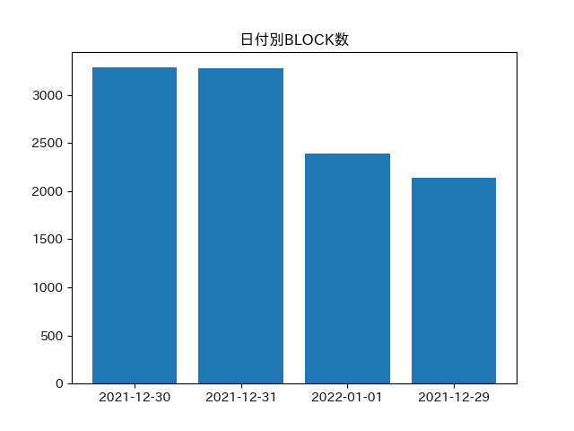
以下は日付別の棒グラフです。
左側が件数です。
12月の30、31は3500件近くありました。
12月の29日は移行日ですので、件数は少ないですね。
1月1日の本日もまだ日中ですので2500件いかないくらい。
1日平均3500弱はブロックしている状況です。
これが公開サーバの恐ろしさですね。
データ部分
日付をカウントするグループを作成し、標準ライブラリのcollectionsで追加、
most_commonで最頻値を特定しています。
        ip_dategroup = collections.Counter(ip_date)

        plt_date_data=[
            ip_dategroup.most_common(1)[0][0],
            ip_dategroup.most_common(2)[1][0],
            ip_dategroup.most_common(3)[2][0],
            ip_dategroup.most_common(4)[3][0],
            ]
        plt_date_ydata=[
            ip_dategroup.most_common(1)[0][1],
            ip_dategroup.most_common(2)[1][1],
            ip_dategroup.most_common(3)[2][1],
            ip_dategroup.most_common(4)[3][1],
            ]
matplotlib箇所
fig = plt.figure()
plt.title('日付別BLOCK数')
plt.bar(plt_date_data,plt_date_ydata)
path3="/share3/backup/pythonlabo/ufwdate.png"
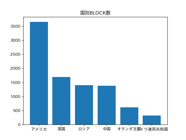
plt.savefig(path3)以下は国別のグラフです。
アメリカがトップ。
他はかなり低めで英国、中国、ロシアが並ぶ感じです。
データ部分
こちらも標準ライブラリのcollectionsで追加、most_commonで最頻値を特定しています。
       ip_cntrgroup = collections.Counter(ip_country)

       plt_cnt_data=[
            ip_cntrgroup.most_common(1)[0][0],
            ip_cntrgroup.most_common(2)[1][0],
            ip_cntrgroup.most_common(3)[2][0],
            ip_cntrgroup.most_common(4)[3][0],
            ip_cntrgroup.most_common(5)[4][0],
            ip_cntrgroup.most_common(6)[5][0],
            ]
        plt_cnt_ydata=[
            ip_cntrgroup.most_common(1)[0][1],
            ip_cntrgroup.most_common(2)[1][1],
            ip_cntrgroup.most_common(3)[2][1],
            ip_cntrgroup.most_common(4)[3][1],
            ip_cntrgroup.most_common(5)[4][1],
            ip_cntrgroup.most_common(6)[5][1],
            ]
matplotlib箇所
fig = plt.figure()
plt.title('国別BLOCK数')
plt.bar(plt_cnt_data,plt_cnt_ydata)
path2="/share3/backup/pythonlabo/ufwcnt.png"
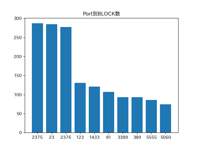
plt.savefig(path2)以下は攻撃対象となったポートのグラフ。
圧倒的にDockerがターゲットにされていますね。
デフォルトのパスワードのままのテンプレ使い回しとかは絶対に狙われそうですね。
データ部分
こちらも標準ライブラリのcollectionsで追加、most_commonで最頻値を特定しています。
        ip_dprtgroup = collections.Counter(ip_dport)

        plt_dprt_data=[
            ip_dprtgroup.most_common(1)[0][0],
            ip_dprtgroup.most_common(2)[1][0],
            ip_dprtgroup.most_common(3)[2][0],
            ip_dprtgroup.most_common(4)[3][0],
            ip_dprtgroup.most_common(5)[4][0],
            ip_dprtgroup.most_common(6)[5][0],
            ip_dprtgroup.most_common(7)[6][0],
            ip_dprtgroup.most_common(8)[7][0],
            ip_dprtgroup.most_common(9)[8][0],
            ip_dprtgroup.most_common(10)[9][0],
            ]
        plt_dprt_ydata=[
            ip_dprtgroup.most_common(1)[0][1],
            ip_dprtgroup.most_common(2)[1][1],
            ip_dprtgroup.most_common(3)[2][1],
            ip_dprtgroup.most_common(4)[3][1],
            ip_dprtgroup.most_common(5)[4][1],
            ip_dprtgroup.most_common(6)[5][1],
            ip_dprtgroup.most_common(7)[6][1],
            ip_dprtgroup.most_common(8)[7][1],
            ip_dprtgroup.most_common(9)[8][1],
            ip_dprtgroup.most_common(10)[9][1],
            ]
matplotlib箇所
       fig = plt.figure()
        plt.title('Port別BLOCK数')
        plt.bar(plt_dprt_data,plt_dprt_ydata)
        path4="/share3/backup/pythonlabo/ufwprt.png"
        plt.savefig(path4)
はい、まずは生成されたグラフと該当コードからご紹介しました。
コード全体
コード全体は以下になります。
集計部分は前回のコードを修正追加したものです。
またログはiptablesのログを使うことにしたため、
余計なログのフィルタリングを追加しています。
for matplot以降がmatplotによるグラフ生成の箇所になります。
#!/usr/bin/python3
import re
import sys
import ipaddress
import geoip2.database
import csv
import collections
import matplotlib.pyplot as plt
import japanize_matplotlib
#filename='/var/log/ufw.log'
filename='/var/log/iptables.log'
ip_address = []
ip_country = []
ip_date = []
ip_dport = []
#gipcity = geoip2.database.Reader("/var/lib/GeoIP/GeoLite2-City.mmdb")
gip = geoip2.database.Reader("/var/lib/GeoIP/GeoLite2-Country.mmdb")

#
def trans_geoip(ip_addr):
    if '192.168.1.' in ip_addr:
        return ('Private')
    try:
        response = gip.country(ip_addr)
        return (response.country.names['ja'])
    except:
        #print('')
        return
#
def trans_word(input_text):
    replacements = {
            'Jan':'01',
            'Feb':'02',
            'Mar':'03',
            'Apl':'04',
            'May':'05',
            'Jun':'06',
            'Jul':'07',
            'Aug':'08',
            'Sep':'09',
            'Oct':'10',
            'Nov':'11',
            'Dec':'12',
            }
#    print('({})'.format('|'.join(map(re.escape,replacements.keys()))))
    return re.sub('({})'.format('|'.join(map(re.escape,replacements.keys()))),lambda m: replacements[m.group()],input_text)
#
if __name__ == '__main__':

    with open(filename) as f:
        reader = csv.reader(f,delimiter=" ",doublequote=False,lineterminator="\r\n")
        for row in reader:
            if row[6]=='ALLOW]':
                #len(row[6])
                #print(row[6],row[10])
                continue
            if row[6]=='AUDIT]':
                #len(row[6])
                #print(row[6],row[10])
                continue
            if row[0]=='Dec':
                if (len(row))>19:
                   # print(row[19].strip("DPT="))
                    ip_dport.append(row[19].strip("DPT="))
                    #if row[10].find('DST=192.168.1.') == True:
                    ip_list = ("2021"+"-"+trans_word(row[0])+"-"+row[1].zfill(2),row[2].zfill(2),row[10].strip("SRC="))
                    ip_address.append(row[10].strip("SRC="))
                    ip_date.append("2021"+"-"+trans_word(row[0])+"-"+row[1].zfill(2))
                   #print(row[10])
                    ip_country.append(trans_geoip(row[10].strip("SRC=")))

            if row[0]!='Dec':
#              f print(row[0][0:10])
                if (len(row))>17:
                    #print(row[17].strip("DPT="))
                    ip_dport.append(row[17].strip("DPT="))
                ip_list = ((row[0][0:10]),row[8].strip("SRC="))
                ip_address.append(row[8].strip("SRC="))
                ip_date.append((row[0][0:10]))
                ip_country.append(trans_geoip(row[8].strip("SRC=")))

        ip_addrgroup = collections.Counter(ip_address)
        ip_dategroup = collections.Counter(ip_date)
        ip_cntrgroup = collections.Counter(ip_country)
        ip_dprtgroup = collections.Counter(ip_dport)
        print(ip_cntrgroup.most_common(10))
        print(ip_dategroup.most_common(10))
        print(ip_addrgroup.most_common(10))
        print(ip_dprtgroup.most_common(10))
        print(len(ip_addrgroup))
        print(trans_geoip(ip_addrgroup.most_common(1)[0][0]),ip_addrgroup.most_common(1)[0][0],ip_addrgroup.most_common(1)[0][1])

######################
#       for matplot
        plt_dprt_data=[
            ip_dprtgroup.most_common(1)[0][0],
            ip_dprtgroup.most_common(2)[1][0],
            ip_dprtgroup.most_common(3)[2][0],
            ip_dprtgroup.most_common(4)[3][0],
            ip_dprtgroup.most_common(5)[4][0],
            ip_dprtgroup.most_common(6)[5][0],
            ip_dprtgroup.most_common(7)[6][0],
            ip_dprtgroup.most_common(8)[7][0],
            ip_dprtgroup.most_common(9)[8][0],
            ip_dprtgroup.most_common(10)[9][0],
            ]
        plt_dprt_ydata=[
            ip_dprtgroup.most_common(1)[0][1],
            ip_dprtgroup.most_common(2)[1][1],
            ip_dprtgroup.most_common(3)[2][1],
            ip_dprtgroup.most_common(4)[3][1],
            ip_dprtgroup.most_common(5)[4][1],
            ip_dprtgroup.most_common(6)[5][1],
            ip_dprtgroup.most_common(7)[6][1],
            ip_dprtgroup.most_common(8)[7][1],
            ip_dprtgroup.most_common(9)[8][1],
            ip_dprtgroup.most_common(10)[9][1],
            ]
        plt_date_data=[
            ip_dategroup.most_common(1)[0][0],
            ip_dategroup.most_common(2)[1][0],
            ip_dategroup.most_common(3)[2][0],
            ip_dategroup.most_common(4)[3][0],
            ]
        plt_date_ydata=[
            ip_dategroup.most_common(1)[0][1],
            ip_dategroup.most_common(2)[1][1],
            ip_dategroup.most_common(3)[2][1],
            ip_dategroup.most_common(4)[3][1],
            ]
        plt_cnt_data=[
            ip_cntrgroup.most_common(1)[0][0],
            ip_cntrgroup.most_common(2)[1][0],
            ip_cntrgroup.most_common(3)[2][0],
            ip_cntrgroup.most_common(4)[3][0],
            ip_cntrgroup.most_common(5)[4][0],
            ip_cntrgroup.most_common(6)[5][0],
            ]
        plt_cnt_ydata=[
            ip_cntrgroup.most_common(1)[0][1],
            ip_cntrgroup.most_common(2)[1][1],
            ip_cntrgroup.most_common(3)[2][1],
            ip_cntrgroup.most_common(4)[3][1],
            ip_cntrgroup.most_common(5)[4][1],
            ip_cntrgroup.most_common(6)[5][1],
            ]
        plt_ip_data=[
            trans_geoip(ip_addrgroup.most_common(1)[0][0]),
            trans_geoip(ip_addrgroup.most_common(2)[1][0]),
            trans_geoip(ip_addrgroup.most_common(3)[2][0]),
            trans_geoip(ip_addrgroup.most_common(4)[3][0]),
            trans_geoip(ip_addrgroup.most_common(5)[4][0]),
            trans_geoip(ip_addrgroup.most_common(6)[5][0]),
            ]
        plt_ip_ydata=[
            ip_addrgroup.most_common(1)[0][1],
            ip_addrgroup.most_common(2)[1][1],
            ip_addrgroup.most_common(3)[2][1],
            ip_addrgroup.most_common(4)[3][1],
            ip_addrgroup.most_common(5)[4][1],
            ip_addrgroup.most_common(6)[5][1],
            ]

        fig = plt.figure()
        plt.title('日付別BLOCK数')
        plt.bar(plt_date_data,plt_date_ydata)
        path3="/share3/backup/pythonlabo/ufwdate.png"
        plt.savefig(path3)

        fig = plt.figure()
        plt.title('国別IP_BLOCK数')
        plt.bar(plt_ip_data,plt_ip_ydata)
        path1="/share3/backup/pythonlabo/ufwip.png"
        plt.savefig(path1)

        fig = plt.figure()
        plt.title('国別BLOCK数')
        plt.bar(plt_cnt_data,plt_cnt_ydata)
        path2="/share3/backup/pythonlabo/ufwcnt.png"
        plt.savefig(path2)

        fig = plt.figure()
        plt.title('Port別BLOCK数')
        plt.bar(plt_dprt_data,plt_dprt_ydata)
        path4="/share3/backup/pythonlabo/ufwprt.png"
        plt.savefig(path4)
matplotへY軸、X軸のデータを投入する箇所については関数化すれば、
もっと効率良いコードになるかと思いますが、今回は単純なコードの繰り返しで作成しています。
まとめ
今回はufwのログをpythonで集計して、matplotlibで棒グラフの作成について紹介しました。
何かの参考になれば幸いです。